Cellular Automata
What are cellular automata?
Cellular automata are simple programs that repetitively apply a rule or set of rules to a grid of cells. Each cell has a state and this state is interpreted by the rules and is altered by the rules. The cells can be arranged in one or more dimensions although they are usually displayed in two dimensions on a computer screen. The state is usually indicated on the computer screen by a particular color. For example if the state of a cell can be either zero or one, a cell with a state of zero may be colored white and a cell with a state of one may be colored black.
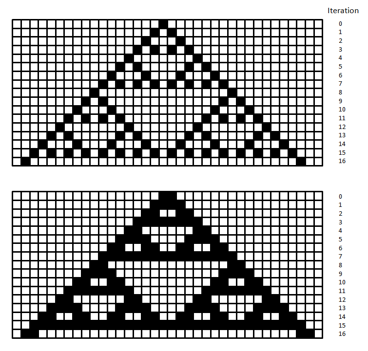
The rules examine the state of a cell and its neighbors and then determine the new state of the cell. For example consider a one dimensional automaton and three pixels or cells in a row. A rule might set the center cell to a value of zero if both neighbors have the same state; otherwise the rule sets the cell’s state to one if they differ. The figure below demonstrates these rules for two different sets of initial condition. Each row of cells represents a single iteration.
Cellular automata do not usually produce fractals or even aesthetically pleasing images but they are interesting because simple rules can produce relatively complex behavior. An example is Conway’s game of life where little blobs move across the screen, sometimes dying, sometimes multiplying. One particular cellular automata algorithm that can produce very detailed images was originally published because it mimics the Belousov-Zhabotinsky chemical reaction. At the time of this writing, all of the cellular automata on this site were produced using this algorithm or a variant of it.
Belousov-Zhabotinsky reaction
The Belousov-Zhabotinsky reaction is a chemical reaction involving bromine and acids that results in oscillations of colored patterns in solution. This chemical reaction of itself is of interest because it demonstrates non-equilibrium thermodynamics. For more details check out the links below:
Chemical oscillations: The Belousov-Zhabotinsky reaction
Wikipedia
Scholarpedia
Belousov-Zhabotinsky Cellular Automaton
This cellular automaton was originally published by A.K. Dewdney (A.K. Dewdney. The hodgepodge machine makes waves. Scientific American. August 1988. p. 104). It’s a 2 dimensional cellular automaton.
A cell can have any of n discrete states where the states are described as follows: a state of zero is considered healthy; a state of n is considered ill; and a state from 1 to n-1 is considered infected.
1) If a cell is healthy (0) then the new state is given by:
a/k1 + b/k2
2) If a cell is ill (n) then the new state of the cell is healthy.
3) And if the cell is infected (1 to n-1) the state given by:
(s/a+b+1) + g
Where:
- a = number of infected neighbors
- b = number of ill neighbors
- k1, k2, and g are constants
- s is the sum of states of the cell and all of its neighbors
There are a number of factors that can affect the results; one obviously is the value of the constants. Below are some examples of the Belousov-Zhabotinsky algorithm with different values of the three constants. Each uses a 3 by 3 grid of cells. That is the center cell has 8 neighbors. Note different color palettes are used with each.
The previous examples used all eight surrounding neighbors. You can also increase the grid to larger squares such as a 5x5 grid or larger. I’ve gone up a 15x15 grid of neighboring cells. You can also exclude cells within the square grid from being considered neighbors. The following examples use patterns of neighboring cells in a 3x3 grid. That is they consider some of the cells within the square grid neighbors and not others. This is indicated for each image by the grid on the right where the cells with an ‘X’ are counted as neighbors and the others are ignored.
In the last example the value of the center cell is multiplied by 3.
The initial seeding also has a big effect. The seeding refers to the initial state or color values of the cells before the automaton is run. Typically each cell is given a random state that is within the color range for the automaton. That is if 256 colors are being used, a single cell will be randomly assigned a value between 1 and 256. But the distribution does not have to be random. Some values can occur more or less frequently than others. Also shapes, patterns and even complex images can be used for the initial image. If the same rules are applied to different random seedings, the resulting images can be very different. The following images show two automata with the same parameters, run for 50 iterations but with different random seedings.
Automata also evolve with each iteration. Some will change for a finite number of cycles and then become fixed but some seem to continue to change no matter how many iterations occur. And some automaton seem to result in a few images that continue to repeat over and over again. This is characteristic of chaotic behavior. The next 3 images show the last automaton run for 100, 152 and 153 iterations.
As mentioned earlier, the initial seeding can have a dramatic affect on the resulting image. The following pairs of images show the results from two different types of initial seedings. In the first pair the left image shows the initial image with the pixels assigned random colors. The right image shows the resulting image.
The next pair shows an initial image seeded with lines. The right image is the resulting image calculated with the same parameters as used in the preceding example.
Even with a single algorithm there are an infinite number of interesting images that can result.